Processing Blocks in a Machine Learning Workflow

Using the example of microspeech

In this post, we look at the creation of an example processing block in a real machine learning workflow. The application we focus on is keyword detection, and the model combines a spectrogram computer with a CNN. The original spectrogram computer is implemented in C-code, and we translate it into Rune processing blocks for deployment as Runes on tiny edge devices.

Machine learning workflows

Machine learning workflows typically have the following steps:

• prepare dataset

• train model

• deploy model

In order to successfully run a deployed model on the edge, the input has to be processed on the deployment in the same way as during the training of the model. Therefore, consistency is required across the whole pipeline - the same operators have to be used during deployment as used during training.

To achieve that for an existing model, there are two options:

1. Match the preprocessing function and distribution of the new data with that of the originally trained model

2. Re-calibrate the model using the preprocessing function used in the deployment and using data drawn from the distribution encountered in the deployment scenario

In this post, we first match the C/C++ implementation of the TensorFlow experimental microspeech frontend op, and then introduce the process of retraining the model with the new processing block.

The keyword recognition model

The model consists of two parts:

1. Spectrogram computer

2. Convolutional Neural Network (CNN)

The spectrogram computer

The spectrogram is computed using a six-step process, using the code in the TensorFlow repo implementing a TensorFlow op micro_frontend:

1. Windowing - implemented in window.c. Takes as input a 1-second audio wav clip: 16000 elements, sampled at 16 kHz. Chops it into 49 windows of 480-elements (30 ms). Gives as output an array of (49, 480).

2. FFT, applied on each window - implemented in fft.cc. Gives as output a (49, 241) array for the frequency responses of each window.

3. Filterbank calculations - implemented in filterbank.c. Aggregates the frequency responses into a smaller set (40) frequency bins, resulting in an array (49, 40).

4. Noise reduction - implemented in noise_reduction.c. Reduces noise within each frequency bin (channel).

5. Auto Gain Control - implemented in pcan_gain_control.c. Applies a gain control algorithm to each frequency bin (channel).

6. Logarithmic scaling - implemented in log_scale.c. Applies log2 function and scales the output.

This provides a lightweight FFT computation library for running on-device. Each of the steps is called in frontend.c, and the Python interface to the TensorFlow op is seen in audio_microfrontend_op.py.

The Convolutional Neural Network (CNN)

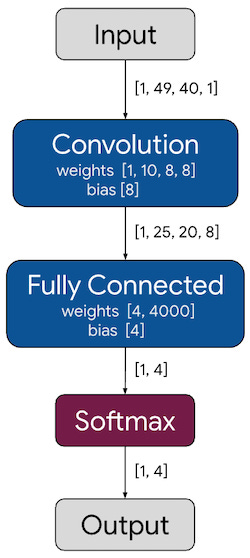
The CNN takes as input the int8 output of the spectrogram computer and gives as output a 4-element vector showing the probability predicted by the model for each of the outcomes (“silence” / “unknown” / “yes” / “no”).

The CNN is a simple model with one convolution and one fully connected layer, implemented as a TFLite model with 8-bit quantized weights.

Deploying the model as a rune container

To deploy the model as a rune container, we need to implement the pre- and post-processing operations as Rune processing blocks.

In this case, we use three processing blocks:

1. fft - combines steps 1-3 of the TensorFlow repo

2. noise-filtering - combines steps 4-6 of the TensorFlow repo

3. ohv_label - translates the output from the CNN model to strings (“silence” / “unknown” / “yes” / “no”)

FROM runicos/base

CAPABILITY<I16[16000]> audio SOUND --hz 16000
PROC_BLOCK<I16[16000],U32[1960]> fft hotg-ai/rune#proc_blocks/fft
PROC_BLOCK<U32[1960],I8[1960]> noise_filtering hotg-ai/rune#proc_blocks/noise-filtering
MODEL<I8[1960],I8[4]> model ./model.tflite

PROC_BLOCK<I8[4],UTF8> label hotg-ai/rune#proc_blocks/ohv_label --labels=silence,unknown,yes,no

OUT serial

RUN audio fft noise_filtering model label serial

The processing blocks are implemented under hotg Rune repo proc_blocks folder. We will focus on two here: FFT, and noise filtering.

The FFT Proc Block

The FFT Proc Block implements the following steps:

• Spectrogram computation (windowing + FFT) using a slightly modified version of the sonogram crate. This gives a (241, 49) dimensional output.

• Mel-spectrum computation using the mel crate. This gives a (40, 49) dimensional output.

• Scaling of the output to [0, 2^32] range (full range of the u32 type). The output will be a vector of 1960 u32 elements.

impl ShortTimeFourierTransform {
    pub const fn new() -> Self {
        ShortTimeFourierTransform {
            sample_rate: DEFAULT_SAMPLE_RATE,
            bins: DEFAULT_BINS,
            window_overlap: DEFAULT_WINDOW_OVERLAP,
        }
    }

    fn transform_inner(&mut self, input: Vec<i16>) -> [u32; 1960] {
        // Build the spectrogram computation engine
        let mut spectrograph = SpecOptionsBuilder::new(49, 241)
            .set_window_fn(sonogram::hann_function)
            .load_data_from_memory(input, self.sample_rate as u32)
            .build();

        // Compute the spectrogram giving the number of bins in a window and the
        // overlap between neighbour windows.
        spectrograph.compute(self.bins, self.window_overlap);

        let spectrogram = spectrograph.create_in_memory(false);

        let filter_count: usize = 40;
        let power_spectrum_size = 241;
        let window_size = 480;
        let sample_rate_usize: usize = 16000;

        // build up the mel filter matrix
        let mut mel_filter_matrix =
            DMatrix::<f64>::zeros(filter_count, power_spectrum_size);
        for (row, col, coefficient) in mel::enumerate_mel_scaling_matrix(
            sample_rate_usize,
            window_size,
            power_spectrum_size,
            filter_count,
        ) {
            mel_filter_matrix[(row, col)] = coefficient;
        }

        let spectrogram = spectrogram.into_iter().map(f64::from);
        let power_spectrum_matrix_unflipped: DMatrix<f64> =
            DMatrix::from_iterator(49, power_spectrum_size, spectrogram);
        let power_spectrum_matrix_transposed =
            power_spectrum_matrix_unflipped.transpose();
        let mut power_spectrum_vec: Vec<_> =
            power_spectrum_matrix_transposed.row_iter().collect();
        &power_spectrum_vec.reverse();
        let power_spectrum_matrix: DMatrix<f64> =
            DMatrix::from_rows(&power_spectrum_vec);
        let mel_spectrum_matrix = &mel_filter_matrix * &power_spectrum_matrix;
        let mel_spectrum_matrix = mel_spectrum_matrix.map(|energy| libm::sqrt(energy));

        let min_value = mel_spectrum_matrix
            .data
            .as_vec()
            .iter()
            .fold(f64::INFINITY, |a, &b| a.min(b));
        let max_value = mel_spectrum_matrix
            .data
            .as_vec()
            .iter()
            .fold(f64::NEG_INFINITY, |a, &b| a.max(b));

        let res: Vec<u32> = mel_spectrum_matrix
            .data
            .as_vec()
            .iter()
            .map(|freq| {
                65536.0 * (freq - min_value) / (max_value - min_value)
            })
            .map(|freq| freq as u32)
            .collect();
        let mut out = [0; 1960];

        for i in 0..1960 {
            out[i] = res[i];
        }

        return out;
    }
}

The Noise Filtering Proc Block

The Noise Filtering Proc Block implements steps 4-6 of the TensorFlow spectrogram computer:

4. Channel-wise smoothing

5. Gain control

6. Log-scaling

The processing block takes as input a 1960-element u32 slice and gives as output a 1960-element i8 slice.

#![no_std]

extern crate alloc;

#[macro_use]
mod macros;
mod gain_control;
mod noise_reduction;

pub use noise_reduction::NoiseReduction;
pub use gain_control::GainControl;

use runic_types::{HasOutputs, Tensor, Transform};

#[derive(Debug, Default, Clone, PartialEq)]
pub struct NoiseFiltering {
    gain_control: GainControl,
    noise_reduction: NoiseReduction,
}

impl NoiseFiltering {
    defered_builder_methods! {
        gain_control.strength: f32;
        gain_control.offset: f32;
        gain_control.gain_bits: i32;
        noise_reduction.smoothing_bits: u32;
        noise_reduction.even_smoothing: f32;
        noise_reduction.odd_smoothing: f32;
        noise_reduction.min_signal_remaining: f32;
    }
}

impl Transform<Tensor<u32>> for NoiseFiltering {
    type Output = Tensor<i8>;

    fn transform(&mut self, input: Tensor<u32>) -> Tensor<i8> {

        let cleaned = self.noise_reduction.transform(input);

        let amplified = self
            .gain_control
            .transform(cleaned, &self.noise_reduction.noise_estimate())
            .map(|_, energy| libm::log2((*energy as f64) + 1.0));

        let min_value = amplified.elements()
            .to_vec()
            .iter()
            .fold(f64::INFINITY, |a, &b| a.min(b));

        let max_value = amplified.elements()
            .to_vec()
            .iter()
            .fold(f64::NEG_INFINITY, |a, &b| a.max(b));

        let scaled = amplified.map(|_, energy| ((255.0 * (energy - min_value) / 
            (max_value - min_value)) - 128.0) as i8);
        scaled

    }
}

Results of the matching

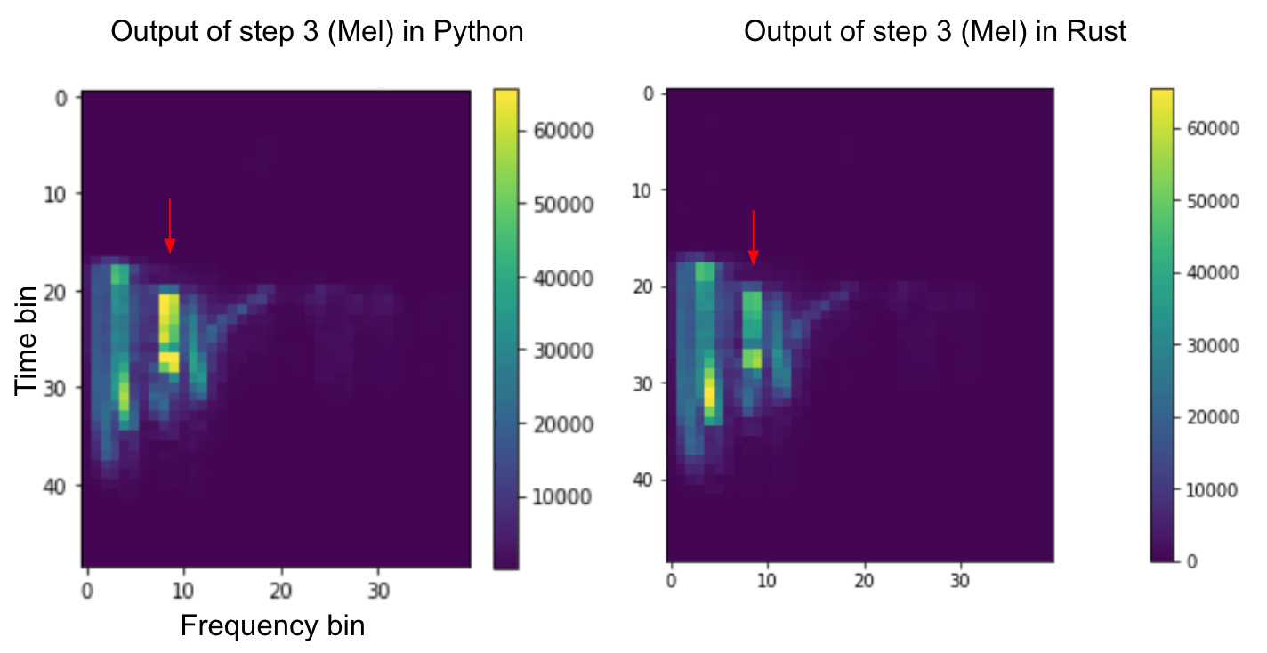
We compare the match between the Python and Rust versions of the spectrogram computer based on an example file containing the utterance “no”. At first, we compare the output of the FFT part in Python and sonogram crate, and see a small difference:

This small difference translates to a difference in the output of step 3, for Mel-spectrogram:

… and this error is amplified further and combined with any implementation differences in the rest of the algorithm (smoothing, gain control, scaling):

The result is that the model trained with the TensorFlow op (left) performs poorer when fed spectrograms for which the model has not been calibrated.

Re-calibrating the CNN model

The model might need to be recalibrated either to adapt to any differences in processing block compared with the original processing block or to adapt the weights to a new person or task.

The TFLITE model can be recalibrated using the associated TensorFlow colab, by replacing the implementation of the spectrogram computer with the Rust version in the training code. More information on calibration and how it is eased by hotg tools will be released in a follow-up post.